pacman::p_load(readr, sf, tmap, spatstat, sfdep, tidyverse, maptools, raster, SpatialAcc, ggstatsplot, reshape2, rgdal, spNetwork)R Packages
Import Data
Aspatial Data
General Practitioner Clinics
gp_data <- read_csv("data/aspatial/gp_data_geocoded.csv")[,-1]Rows: 1221 Columns: 7
── Column specification ────────────────────────────────────────────────────────
Delimiter: ","
chr (2): clinic, postal_code
dbl (5): index, X, Y, Lat, Long
ℹ Use `spec()` to retrieve the full column specification for this data.
ℹ Specify the column types or set `show_col_types = FALSE` to quiet this message.head(gp_data, 5)# A tibble: 5 × 6
clinic postal_code X Y Lat Long
<chr> <chr> <dbl> <dbl> <dbl> <dbl>
1 RafflesMedical 159953 24849. 30114. 1.29 104.
2 Shenton Medical Group 119963 24433. 28496. 1.27 104.
3 Town Hall Clinic 119967 24375. 28917. 1.28 104.
4 Chuah Clinic & Surgery 380113 33881. 33643. 1.32 104.
5 ECM Clinic & Surgery 387604 33518. 33021. 1.31 104.Hospitals
hospital_data <- read_csv("data/aspatial/hospital_data_geocoded.csv")Rows: 27 Columns: 11
── Column specification ────────────────────────────────────────────────────────
Delimiter: ","
chr (6): HOSPITAL_NAME, PRIVATE, TYPE, MANAGED_BY, ADDRESS, NUM_OF_BEDS
dbl (5): POSTAL_CODE, X, Y, Lat, Long
ℹ Use `spec()` to retrieve the full column specification for this data.
ℹ Specify the column types or set `show_col_types = FALSE` to quiet this message.head(hospital_data, 5)# A tibble: 5 × 11
HOSPITAL_N…¹ PRIVATE TYPE MANAG…² ADDRESS POSTA…³ NUM_O…⁴ X Y Lat
<chr> <chr> <chr> <chr> <chr> <dbl> <chr> <dbl> <dbl> <dbl>
1 ALEXANDRA H… Y GENE… <NA> ALEXAN… 159964 176 24230. 30060. 1.29
2 BRIGHT VISI… N COMM… SINGHE… 5 LORO… 547530 317 32976. 39338. 1.37
3 CHANGI GENE… N GENE… SINGHE… 2 SIME… 529889 1,000 40784. 35942. 1.34
4 CONCORD INT… Y SPEC… <NA> 19 Ada… 289891 34 25774. 34337. 1.33
5 FARRER PARK… Y GENE… <NA> 1 Farr… 217562 121 30284. 32783. 1.31
# … with 1 more variable: Long <dbl>, and abbreviated variable names
# ¹HOSPITAL_NAME, ²MANAGED_BY, ³POSTAL_CODE, ⁴NUM_OF_BEDSPolyclinics
poly_data <- read_csv("data/aspatial/polyclinic_data_geocoded.csv")Rows: 20 Columns: 8
── Column specification ────────────────────────────────────────────────────────
Delimiter: ","
chr (3): POLYCLINIC, MANAGED_BY, ADDRESS
dbl (5): POSTAL_CODE, X, Y, Lat, Long
ℹ Use `spec()` to retrieve the full column specification for this data.
ℹ Specify the column types or set `show_col_types = FALSE` to quiet this message.head(poly_data, 5)# A tibble: 5 × 8
POLYCLINIC MANAGED_BY ADDRESS POSTA…¹ X Y Lat Long
<chr> <chr> <chr> <dbl> <dbl> <dbl> <dbl> <dbl>
1 ANG MO KIO POLYCLINIC NHG 21 ANG … 569666 29375. 39591. 1.37 104.
2 BEDOK POLYCLINIC Singhealth HEARTBE… 469662 38997. 34344. 1.33 104.
3 BUKIT BATOK POLYCLINIC NUHS 50 BUKI… 659164 18485. 37125. 1.35 104.
4 BUKIT MERAH POLYCLINIC Singhealth 163 BUK… 150163 26192. 29566. 1.28 104.
5 CHOA CHU KANG POLYCLINIC NUHS 2 TECK … 688846 18814. 40478. 1.38 104.
# … with abbreviated variable name ¹POSTAL_CODENursing Homes
nursing_data <- read_csv("data/aspatial/nursing_home_data_geocoded.csv")Rows: 76 Columns: 7
── Column specification ────────────────────────────────────────────────────────
Delimiter: ","
chr (2): NURSING_HOME_NAME, ADDRESS
dbl (5): POSTAL_CODE, X, Y, Lat, Long
ℹ Use `spec()` to retrieve the full column specification for this data.
ℹ Specify the column types or set `show_col_types = FALSE` to quiet this message.head(nursing_data, 5)# A tibble: 5 × 7
NURSING_HOME_NAME ADDRESS POSTA…¹ X Y Lat Long
<chr> <chr> <dbl> <dbl> <dbl> <dbl> <dbl>
1 ALL SAINTS HOME (HOUGANG) 5 Poh Huat Ro… 546703 33636. 38608. 1.37 104.
2 ALL SAINTS HOME (JURONG EAST) 20 JURONG EAS… 609792 17702. 35990. 1.34 104.
3 ALL SAINTS HOME (TAMPINES) 11 TAMPINES S… 529123 41443. 38141. 1.36 104.
4 ALL SAINTS HOME (YISHUN) 551 YISHUN RI… 768681 27662. 46348. 1.44 104.
5 APEX HARMONY LODGE 10 PASIR RIS … 518240 42573. 39170. 1.37 104.
# … with abbreviated variable name ¹POSTAL_CODEPrimary Care Networks
pcn_data <- read_csv("data/aspatial/PCN Clinic Listing (by PCN) With Postal Code.csv")New names:
Rows: 828 Columns: 19
── Column specification
──────────────────────────────────────────────────────── Delimiter: "," chr
(13): PCN, Clinic Name, Address, Operating Hours (Please call the clinic... dbl
(6): S/N, results.POSTAL...15, results.X, results.Y, results.LATITUDE, ...
ℹ Use `spec()` to retrieve the full column specification for this data. ℹ
Specify the column types or set `show_col_types = FALSE` to quiet this message.
• `results.POSTAL` -> `results.POSTAL...9`
• `results.POSTAL` -> `results.POSTAL...15`head(pcn_data, 5)# A tibble: 5 × 19
`S/N` PCN Clini…¹ Address Opera…² Conta…³ Addre…⁴ Posta…⁵ resul…⁶ resul…⁷
<dbl> <chr> <chr> <chr> <chr> <chr> <chr> <chr> <chr> <chr>
1 1 ASSURAN… 57 MED… BLK 32… "Monda… 651892… BLK 32… 390032 390032 32 CAS…
2 2 ASSURAN… ACUMED… 301 BO… "Monda… 65,159… 301 BO… 649846 649846 BOON L…
3 3 ASSURAN… ACUMED… BLK 21… "Monda… 64,438… BLK 21… 460214 460214 BEDOK …
4 4 ASSURAN… ACUMED… 1 JOO … "Monda… 68,615… 1 JOO … 629117 629117 DBS NT…
5 5 ASSURAN… ACUMED… 1 JURO… "Monda… 67,923… 1 JURO… 648886 648886 OCBC J…
# … with 9 more variables: results.BLK_NO <chr>, results.ROAD_NAME <chr>,
# results.BUILDING <chr>, results.ADDRESS <chr>, results.POSTAL...15 <dbl>,
# results.X <dbl>, results.Y <dbl>, results.LATITUDE <dbl>,
# results.LONGITUDE <dbl>, and abbreviated variable names ¹`Clinic Name`,
# ²`Operating Hours (Please call the clinic before visiting)`, ³`Contact No`,
# ⁴`Address Check`, ⁵`Postal Code`, ⁶results.POSTAL...9, ⁷results.SEARCHVALResident Population by Planning Area/Subzone, Age Group and Sex
Only total population, not separated by genders
pop_data <- read_csv("data/aspatial/Resident Population 2015.csv", skip=11)[1:379,1:58]New names:
Rows: 401 Columns: 59
── Column specification
──────────────────────────────────────────────────────── Delimiter: "," chr
(58): ...1, Total...2, 0 - 4...3, 5 - 9...4, 10 - 14...5, 15 - 19...6, 2... lgl
(1): ...59
ℹ Use `spec()` to retrieve the full column specification for this data. ℹ
Specify the column types or set `show_col_types = FALSE` to quiet this message.
• `` -> `...1`
• `Total` -> `Total...2`
• `0 - 4` -> `0 - 4...3`
• `5 - 9` -> `5 - 9...4`
• `10 - 14` -> `10 - 14...5`
• `15 - 19` -> `15 - 19...6`
• `20 - 24` -> `20 - 24...7`
• `25 - 29` -> `25 - 29...8`
• `30 - 34` -> `30 - 34...9`
• `35 - 39` -> `35 - 39...10`
• `40 - 44` -> `40 - 44...11`
• `45 - 49` -> `45 - 49...12`
• `50 - 54` -> `50 - 54...13`
• `55 - 59` -> `55 - 59...14`
• `60 - 64` -> `60 - 64...15`
• `65 - 69` -> `65 - 69...16`
• `70 - 74` -> `70 - 74...17`
• `75 - 79` -> `75 - 79...18`
• `80 - 84` -> `80 - 84...19`
• `85 & Over` -> `85 & Over...20`
• `Total` -> `Total...21`
• `0 - 4` -> `0 - 4...22`
• `5 - 9` -> `5 - 9...23`
• `10 - 14` -> `10 - 14...24`
• `15 - 19` -> `15 - 19...25`
• `20 - 24` -> `20 - 24...26`
• `25 - 29` -> `25 - 29...27`
• `30 - 34` -> `30 - 34...28`
• `35 - 39` -> `35 - 39...29`
• `40 - 44` -> `40 - 44...30`
• `45 - 49` -> `45 - 49...31`
• `50 - 54` -> `50 - 54...32`
• `55 - 59` -> `55 - 59...33`
• `60 - 64` -> `60 - 64...34`
• `65 - 69` -> `65 - 69...35`
• `70 - 74` -> `70 - 74...36`
• `75 - 79` -> `75 - 79...37`
• `80 - 84` -> `80 - 84...38`
• `85 & Over` -> `85 & Over...39`
• `Total` -> `Total...40`
• `0 - 4` -> `0 - 4...41`
• `5 - 9` -> `5 - 9...42`
• `10 - 14` -> `10 - 14...43`
• `15 - 19` -> `15 - 19...44`
• `20 - 24` -> `20 - 24...45`
• `25 - 29` -> `25 - 29...46`
• `30 - 34` -> `30 - 34...47`
• `35 - 39` -> `35 - 39...48`
• `40 - 44` -> `40 - 44...49`
• `45 - 49` -> `45 - 49...50`
• `50 - 54` -> `50 - 54...51`
• `55 - 59` -> `55 - 59...52`
• `60 - 64` -> `60 - 64...53`
• `65 - 69` -> `65 - 69...54`
• `70 - 74` -> `70 - 74...55`
• `75 - 79` -> `75 - 79...56`
• `80 - 84` -> `80 - 84...57`
• `85 & Over` -> `85 & Over...58`
• `` -> `...59`head(pop_data, 5)# A tibble: 5 × 58
...1 Total…¹ 0 - 4…² 5 - 9…³ 10 - …⁴ 15 - …⁵ 20 - …⁶ 25 - …⁷ 30 - …⁸ 35 - …⁹
<chr> <chr> <chr> <chr> <chr> <chr> <chr> <chr> <chr> <chr>
1 Total 3902690 183580 204450 214390 242900 264130 271030 290620 301070
2 Ang M… 174770 6790 7660 8290 9320 10310 11170 12250 13070
3 Ang M… 5020 260 280 320 280 260 310 370 420
4 Cheng… 29770 1290 1180 1290 1400 1570 1830 2490 2490
5 Chong… 27900 910 1100 1180 1370 1520 1800 1980 2100
# … with 48 more variables: `40 - 44...11` <chr>, `45 - 49...12` <chr>,
# `50 - 54...13` <chr>, `55 - 59...14` <chr>, `60 - 64...15` <chr>,
# `65 - 69...16` <chr>, `70 - 74...17` <chr>, `75 - 79...18` <chr>,
# `80 - 84...19` <chr>, `85 & Over...20` <chr>, Total...21 <chr>,
# `0 - 4...22` <chr>, `5 - 9...23` <chr>, `10 - 14...24` <chr>,
# `15 - 19...25` <chr>, `20 - 24...26` <chr>, `25 - 29...27` <chr>,
# `30 - 34...28` <chr>, `35 - 39...29` <chr>, `40 - 44...30` <chr>, …PCN
pcn_data <- readr::read_csv("data/aspatial/PCN Clinic Listing (by PCN) With Postal Code.csv")New names:
Rows: 828 Columns: 19
── Column specification
──────────────────────────────────────────────────────── Delimiter: "," chr
(13): PCN, Clinic Name, Address, Operating Hours (Please call the clinic... dbl
(6): S/N, results.POSTAL...15, results.X, results.Y, results.LATITUDE, ...
ℹ Use `spec()` to retrieve the full column specification for this data. ℹ
Specify the column types or set `show_col_types = FALSE` to quiet this message.
• `results.POSTAL` -> `results.POSTAL...9`
• `results.POSTAL` -> `results.POSTAL...15`Geospatial Data
Master Plan Subzone 2019
mpsz <- st_read(dsn = "data/geospatial/MPSZ-2019",
layer = "MPSZ-2019") %>%
st_transform(crs = 3414)Reading layer `MPSZ-2019' from data source
`C:\deadline2359\IS415-Project\posts\data_cleaning\data\geospatial\MPSZ-2019'
using driver `ESRI Shapefile'
Simple feature collection with 332 features and 6 fields
Geometry type: MULTIPOLYGON
Dimension: XY
Bounding box: xmin: 103.6057 ymin: 1.158699 xmax: 104.0885 ymax: 1.470775
Geodetic CRS: WGS 84write_rds(mpsz, "data/models/mpsz_original.rds")head(mpsz, 5)Simple feature collection with 5 features and 6 fields
Geometry type: MULTIPOLYGON
Dimension: XY
Bounding box: xmin: 8012.578 ymin: 22108.68 xmax: 33316.59 ymax: 31087.61
Projected CRS: SVY21 / Singapore TM
SUBZONE_N SUBZONE_C PLN_AREA_N PLN_AREA_C REGION_N
1 MARINA EAST MESZ01 MARINA EAST ME CENTRAL REGION
2 INSTITUTION HILL RVSZ05 RIVER VALLEY RV CENTRAL REGION
3 ROBERTSON QUAY SRSZ01 SINGAPORE RIVER SR CENTRAL REGION
4 JURONG ISLAND AND BUKOM WISZ01 WESTERN ISLANDS WI WEST REGION
5 FORT CANNING MUSZ02 MUSEUM MU CENTRAL REGION
REGION_C geometry
1 CR MULTIPOLYGON (((33222.98 29...
2 CR MULTIPOLYGON (((28481.45 30...
3 CR MULTIPOLYGON (((28087.34 30...
4 WR MULTIPOLYGON (((14557.7 304...
5 CR MULTIPOLYGON (((29542.53 31...Eldercare
eldercare_sf <- st_read(dsn = "data/geospatial/eldercare",
layer = "ELDERCARE") %>%
st_transform(crs = 3414)Reading layer `ELDERCARE' from data source
`C:\deadline2359\IS415-Project\posts\data_cleaning\data\geospatial\eldercare'
using driver `ESRI Shapefile'
Simple feature collection with 120 features and 19 fields
Geometry type: POINT
Dimension: XY
Bounding box: xmin: 14481.92 ymin: 28218.43 xmax: 41665.14 ymax: 46804.9
Projected CRS: SVY21 / Singapore TMhead(eldercare_sf, 5)Simple feature collection with 5 features and 19 fields
Geometry type: POINT
Dimension: XY
Bounding box: xmin: 14481.92 ymin: 30135.49 xmax: 38803.81 ymax: 36639.12
Projected CRS: SVY21 / Singapore TM
fid OBJECTID ADDRESSBLO ADDRESSBUI ADDRESSPOS
1 1 1 <NA> <NA> 601318
2 2 2 <NA> <NA> 462509
3 3 3 <NA> <NA> 640190
4 4 4 <NA> <NA> 190005
5 5 5 <NA> <NA> 160044
ADDRESSSTR ADDRESSTYP DESCRIPTIO HYPERLINK
1 318A Jurong East Avenue 1 #02-308 <NA> <NA> <NA>
2 Blk 509B Bedok North Street 3 #02-157 <NA> <NA> <NA>
3 Blk 190 Boon Lay Drive #01-242 <NA> <NA> <NA>
4 5 Beach Rd #02-4943 <NA> <NA> <NA>
5 Blk 44 Beo Crescent #01-67 <NA> <NA> <NA>
LANDXADDRE LANDYADDRE NAME PHOTOURL
1 0 0 Yuhua Senior Activity Centre <NA>
2 0 0 THK SAC @ Kaki Bukit <NA>
3 0 0 THK SAC @ Boon Lay <NA>
4 0 0 PEACE-Connect Senior Activity Centre@5 <NA>
5 0 0 THK SAC @ Beo Crescent <NA>
ADDRESSFLO INC_CRC FMEL_UPD_D ADDRESSUNI X_ADDR Y_ADDR
1 <NA> 2B0DB92FDD914FFC 2016-07-28 <NA> 16614.08 36639.12
2 <NA> 82728FA30612F3FD 2016-07-28 <NA> 38803.81 35098.78
3 <NA> DE7A8D4EA0BD1D9B 2016-07-28 <NA> 14481.92 36357.61
4 <NA> A2C058FC5785F7FE 2016-07-28 <NA> 31505.35 31853.52
5 <NA> 9DBFD51E056AEE70 2016-07-28 <NA> 27218.35 30135.49
geometry
1 POINT (16614.08 36639.12)
2 POINT (38803.81 35098.78)
3 POINT (14481.92 36357.61)
4 POINT (31505.35 31853.52)
5 POINT (27218.35 30135.49)Locations of Bus Stops
busstop_sf <- st_read(dsn = "data/geospatial/BusStop_Feb2023",
layer = "BusStop") %>%
st_transform(crs = 3414)Reading layer `BusStop' from data source
`C:\deadline2359\IS415-Project\posts\data_cleaning\data\geospatial\BusStop_Feb2023'
using driver `ESRI Shapefile'
Simple feature collection with 5159 features and 3 fields
Geometry type: POINT
Dimension: XY
Bounding box: xmin: 3970.122 ymin: 26482.1 xmax: 48284.56 ymax: 52983.82
Projected CRS: SVY21head(busstop_sf, 5)Simple feature collection with 5 features and 3 fields
Geometry type: POINT
Dimension: XY
Bounding box: xmin: 13228.59 ymin: 30391.85 xmax: 41603.76 ymax: 44206.38
Projected CRS: SVY21 / Singapore TM
BUS_STOP_N BUS_ROOF_N LOC_DESC geometry
1 22069 B06 OPP CEVA LOGISTICS POINT (13576.31 32883.65)
2 32071 B23 AFT TRACK 13 POINT (13228.59 44206.38)
3 44331 B01 BLK 239 POINT (21045.1 40242.08)
4 96081 B05 GRACE INDEPENDENT CH POINT (41603.76 35413.11)
5 11561 B05 BLK 166 POINT (24568.74 30391.85)Locations of Train Stations
trainstation_sf <- st_read(dsn = "data/geospatial/TrainStation_Feb2023",
layer = "RapidTransitSystemStation")[,c(-1, -2)] %>%
st_transform(crs = 3414)Reading layer `RapidTransitSystemStation' from data source
`C:\deadline2359\IS415-Project\posts\data_cleaning\data\geospatial\TrainStation_Feb2023'
using driver `ESRI Shapefile'Warning in CPL_read_ogr(dsn, layer, query, as.character(options), quiet, : GDAL
Message 1: Non closed ring detected. To avoid accepting it, set the
OGR_GEOMETRY_ACCEPT_UNCLOSED_RING configuration option to NOSimple feature collection with 220 features and 4 fields
Geometry type: POLYGON
Dimension: XY
Bounding box: xmin: 6068.209 ymin: 27478.44 xmax: 45377.5 ymax: 47913.58
Projected CRS: SVY21head(trainstation_sf, 5)Simple feature collection with 5 features and 2 fields
Geometry type: POLYGON
Dimension: XY
Bounding box: xmin: 29286.74 ymin: 30548.91 xmax: 34623.54 ymax: 33404.47
Projected CRS: SVY21 / Singapore TM
TYP_CD_DES STN_NAM_DE geometry
1 MRT ESPLANADE MRT STATION POLYGON ((30566.07 30621.21...
2 MRT PAYA LEBAR MRT STATION POLYGON ((34495.6 33384.44,...
3 MRT DHOBY GHAUT MRT STATION POLYGON ((29293.51 31312.53...
4 MRT DAKOTA MRT STATION POLYGON ((34055.08 32290.62...
5 MRT LAVENDER MRT STATION POLYGON ((31236.5 32085.76,...CHAS
chas_sf <- st_read(dsn = "data/geospatial/CHAS Clinics Shapefile",
layer = "CHAS Clinics") %>%
st_transform(crs = 3414)Reading layer `CHAS Clinics' from data source
`C:\deadline2359\IS415-Project\posts\data_cleaning\data\geospatial\CHAS Clinics Shapefile'
using driver `ESRI Shapefile'
replacing null geometries with empty geometries
Simple feature collection with 1917 features and 19 fields (with 5 geometries empty)
Geometry type: POINT
Dimension: XY
Bounding box: xmin: 4985.536 ymin: 26424.19 xmax: 45457.14 ymax: 48626.7
Projected CRS: SVY21 / Singapore TMhead(chas_sf, 5)Simple feature collection with 5 features and 19 fields
Geometry type: POINT
Dimension: XY
Bounding box: xmin: 17595.29 ymin: 35041.76 xmax: 33064.94 ymax: 39158.18
Projected CRS: SVY21 / Singapore TM
fid Name
1 1 1 Aljunied Medical
2 2 1 BISHAN MEDICAL
3 3 1 MEDICAL TECK GHEE
4 4 1728 Dental Practice (Ang Mo Kio)
5 5 1728 Dental Practice (Jurong)
Address
1 Singapore 367874
2 283, Bishan Street, #01- 191, Singapore\n570283
3 410, ANG MO KIO AVENUE 10, TECK GHEE SQUARE, #01- 837, Singapore\n560410
4 704, Ang Mo Kio Ave 8, #01- 2559, Singapore 560704
5 135, Jurong Gateway Road, #01- 319,\nSingapore 600135
Telephone Type
1 <NA> Medical, Public Health Preparedness Clinic
2 64561600 Medical, Cervical Cancer Screen, Public Health Preparedness Clinic
3 62517030 Medical
4 96311728 Dental
5 97701728 Dental
Website Pap.Test.S Postal.Cod results.PO
1 <NA> 0 367874 367874
2 <NA> 1 570283 570283
3 <NA> 0 560410 560410
4 <NA> 0 560704 560704
5 <NA> 0 600135 600135
results.SE results.BL results.RO
1 389 UPPER ALJUNIED ROAD SINGAPORE 367874 389 UPPER ALJUNIED ROAD
2 283 BISHAN STREET 22 SINGAPORE 570283 283 BISHAN STREET 22
3 410 ANG MO KIO AVENUE 10 SINGAPORE 560410 410 ANG MO KIO AVENUE 10
4 704 ANG MO KIO AVENUE 8 SINGAPORE 560704 704 ANG MO KIO AVENUE 8
5 OCBC JURONG GATEWAY ROAD - FAIRPRICE 135 JURONG GATEWAY ROAD
results.BU
1 NIL
2 NIL
3 NIL
4 NIL
5 OCBC JURONG GATEWAY ROAD - FAIRPRICE
results.AD
1 389 UPPER ALJUNIED ROAD SINGAPORE 367874
2 283 BISHAN STREET 22 SINGAPORE 570283
3 410 ANG MO KIO AVENUE 10 SINGAPORE 560410
4 704 ANG MO KIO AVENUE 8 SINGAPORE 560704
5 135 JURONG GATEWAY ROAD OCBC JURONG GATEWAY ROAD - FAIRPRICE SINGAPORE 600135
results._1 results.X results.Y results.LA results.LO
1 367874 33064.94 35041.76 1.333179 103.8788
2 570283 29272.03 37887.89 1.358919 103.8447
3 560410 30373.38 38307.67 1.362715 103.8546
4 560704 29548.25 39158.18 1.370407 103.8472
5 600135 17595.29 35116.25 1.333852 103.7398
geometry
1 POINT (33064.94 35041.76)
2 POINT (29272.03 37887.89)
3 POINT (30373.38 38307.67)
4 POINT (29548.25 39158.18)
5 POINT (17595.29 35116.25)chas_sf <- chas_sf[rowSums(is.na(chas_sf)) == 0, ] Data Preparation
#pcn_sf <- st_as_sf(pcn_data, coords=c("results.LONGITUDE", "results.LATITUDE"), crs=4326) %>% st_transform(crs = 3414)
#pcn_data$results.LATITUDE
#pcn_data[is.na(pcn_data$results.LATITUDE),]
chas_sf <- chas_sf[rowSums(is.na(chas_sf)) == 0, ]
pcn_data <- pcn_data[rowSums(is.na(pcn_data)) == 0, ]Retrieve Geospatial Data
General Practitioner Clinics
gp_sf <- st_as_sf(gp_data, coords=c("Long", "Lat"), crs=4326) %>% st_transform(crs = 3414)
gp_sf <- gp_sf[, c(1,2)]head(gp_sf, 5)Simple feature collection with 5 features and 2 fields
Geometry type: POINT
Dimension: XY
Bounding box: xmin: 24374.75 ymin: 28496.49 xmax: 33880.65 ymax: 33642.63
Projected CRS: SVY21 / Singapore TM
# A tibble: 5 × 3
clinic postal_code geometry
<chr> <chr> <POINT [m]>
1 RafflesMedical 159953 (24849.49 30114)
2 Shenton Medical Group 119963 (24432.59 28496.49)
3 Town Hall Clinic 119967 (24374.75 28916.52)
4 Chuah Clinic & Surgery 380113 (33880.65 33642.63)
5 ECM Clinic & Surgery 387604 (33518.21 33021.09)Hospitals
hospital_sf <- st_as_sf(hospital_data, coords=c("Long", "Lat"), crs=4326) %>% st_transform(crs = 3414)
hospital_sf <- hospital_sf[, c(1:7)]head(hospital_sf, 5)Simple feature collection with 5 features and 7 fields
Geometry type: POINT
Dimension: XY
Bounding box: xmin: 24230.14 ymin: 30059.55 xmax: 40784.33 ymax: 39338.44
Projected CRS: SVY21 / Singapore TM
# A tibble: 5 × 8
HOSPITAL_NAME PRIVATE TYPE MANAG…¹ ADDRESS POSTA…² NUM_O…³
<chr> <chr> <chr> <chr> <chr> <dbl> <chr>
1 ALEXANDRA HOSPITAL Y GENERAL <NA> ALEXAN… 159964 176
2 BRIGHT VISION HOSPITAL N COMMUN… SINGHE… 5 LORO… 547530 317
3 CHANGI GENERAL HOSPITAL N GENERAL SINGHE… 2 SIME… 529889 1,000
4 CONCORD INTERNATIONAL HOSPITAL Y SPECIA… <NA> 19 Ada… 289891 34
5 FARRER PARK HOSPITAL Y GENERAL <NA> 1 Farr… 217562 121
# … with 1 more variable: geometry <POINT [m]>, and abbreviated variable names
# ¹MANAGED_BY, ²POSTAL_CODE, ³NUM_OF_BEDSPolyclinics
poly_sf <- st_as_sf(poly_data, coords=c("Long", "Lat"), crs=4326) %>% st_transform(crs = 3414)
poly_sf <- poly_sf[, c(1:4)]head(poly_sf, 5)Simple feature collection with 5 features and 4 fields
Geometry type: POINT
Dimension: XY
Bounding box: xmin: 18485.22 ymin: 29566.29 xmax: 38996.66 ymax: 40477.96
Projected CRS: SVY21 / Singapore TM
# A tibble: 5 × 5
POLYCLINIC MANAGED_BY ADDRESS POSTA…¹ geometry
<chr> <chr> <chr> <dbl> <POINT [m]>
1 ANG MO KIO POLYCLINIC NHG 21 ANG … 569666 (29375.43 39591.35)
2 BEDOK POLYCLINIC Singhealth HEARTBE… 469662 (38996.66 34343.66)
3 BUKIT BATOK POLYCLINIC NUHS 50 BUKI… 659164 (18485.22 37124.65)
4 BUKIT MERAH POLYCLINIC Singhealth 163 BUK… 150163 (26191.96 29566.29)
5 CHOA CHU KANG POLYCLINIC NUHS 2 TECK … 688846 (18814.15 40477.96)
# … with abbreviated variable name ¹POSTAL_CODENursing Homes
nursing_sf <- st_as_sf(nursing_data, coords=c("Long", "Lat"), crs=4326) %>% st_transform(crs = 3414)
nursing_sf <- nursing_sf[, c(1:3)]head(nursing_sf, 5)Simple feature collection with 5 features and 3 fields
Geometry type: POINT
Dimension: XY
Bounding box: xmin: 17702.24 ymin: 35989.84 xmax: 42573.31 ymax: 46347.74
Projected CRS: SVY21 / Singapore TM
# A tibble: 5 × 4
NURSING_HOME_NAME ADDRESS POSTA…¹ geometry
<chr> <chr> <dbl> <POINT [m]>
1 ALL SAINTS HOME (HOUGANG) 5 Poh Huat Ro… 546703 (33635.6 38608.27)
2 ALL SAINTS HOME (JURONG EAST) 20 JURONG EAS… 609792 (17702.24 35989.84)
3 ALL SAINTS HOME (TAMPINES) 11 TAMPINES S… 529123 (41443.41 38141.06)
4 ALL SAINTS HOME (YISHUN) 551 YISHUN RI… 768681 (27662.47 46347.74)
5 APEX HARMONY LODGE 10 PASIR RIS … 518240 (42573.31 39170.3)
# … with abbreviated variable name ¹POSTAL_CODEPrimary Care Network
pcn_sf <- st_as_sf(pcn_data, coords=c("results.LONGITUDE", "results.LATITUDE"), crs=4326) %>% st_transform(crs = 3414)
pcn_sf <- pcn_sf[, c(2:6, 8)]Data
head(pcn_sf, 5)Simple feature collection with 5 features and 6 fields
Geometry type: POINT
Dimension: XY
Bounding box: xmin: 10725.31 ymin: 32414.15 xmax: 39037.12 ymax: 35735.68
Projected CRS: SVY21 / Singapore TM
# A tibble: 5 × 7
PCN Clini…¹ Address Opera…² Conta…³ Posta…⁴ geometry
<chr> <chr> <chr> <chr> <chr> <chr> <POINT [m]>
1 ASSURANCE P… 57 MED… BLK 32… "Monda… 651892… 390032 (33629.25 32414.15)
2 ASSURANCE P… ACUMED… 301 BO… "Monda… 65,159… 649846 (13813.58 35629.67)
3 ASSURANCE P… ACUMED… BLK 21… "Monda… 64,438… 460214 (39037.12 34234.33)
4 ASSURANCE P… ACUMED… 1 JOO … "Monda… 68,615… 629117 (10725.31 34094.33)
5 ASSURANCE P… ACUMED… 1 JURO… "Monda… 67,923… 648886 (13907.03 35735.68)
# … with abbreviated variable names ¹`Clinic Name`,
# ²`Operating Hours (Please call the clinic before visiting)`, ³`Contact No`,
# ⁴`Postal Code`:::
Merge MPSZ with Population Data
Convert Data Types
pop_is_char <- sapply(pop_data[c(2:58)], is.character)
pop_data[c(2:58)][ , pop_is_char] <- as.data.frame(apply(pop_data[c(2:58)][ , pop_is_char], 2, as.numeric))Warning in apply(pop_data[c(2:58)][, pop_is_char], 2, as.numeric): NAs
introduced by coercion
Warning in apply(pop_data[c(2:58)][, pop_is_char], 2, as.numeric): NAs
introduced by coercion
Warning in apply(pop_data[c(2:58)][, pop_is_char], 2, as.numeric): NAs
introduced by coercion
Warning in apply(pop_data[c(2:58)][, pop_is_char], 2, as.numeric): NAs
introduced by coercion
Warning in apply(pop_data[c(2:58)][, pop_is_char], 2, as.numeric): NAs
introduced by coercion
Warning in apply(pop_data[c(2:58)][, pop_is_char], 2, as.numeric): NAs
introduced by coercion
Warning in apply(pop_data[c(2:58)][, pop_is_char], 2, as.numeric): NAs
introduced by coercion
Warning in apply(pop_data[c(2:58)][, pop_is_char], 2, as.numeric): NAs
introduced by coercion
Warning in apply(pop_data[c(2:58)][, pop_is_char], 2, as.numeric): NAs
introduced by coercion
Warning in apply(pop_data[c(2:58)][, pop_is_char], 2, as.numeric): NAs
introduced by coercion
Warning in apply(pop_data[c(2:58)][, pop_is_char], 2, as.numeric): NAs
introduced by coercion
Warning in apply(pop_data[c(2:58)][, pop_is_char], 2, as.numeric): NAs
introduced by coercion
Warning in apply(pop_data[c(2:58)][, pop_is_char], 2, as.numeric): NAs
introduced by coercion
Warning in apply(pop_data[c(2:58)][, pop_is_char], 2, as.numeric): NAs
introduced by coercion
Warning in apply(pop_data[c(2:58)][, pop_is_char], 2, as.numeric): NAs
introduced by coercion
Warning in apply(pop_data[c(2:58)][, pop_is_char], 2, as.numeric): NAs
introduced by coercion
Warning in apply(pop_data[c(2:58)][, pop_is_char], 2, as.numeric): NAs
introduced by coercion
Warning in apply(pop_data[c(2:58)][, pop_is_char], 2, as.numeric): NAs
introduced by coercion
Warning in apply(pop_data[c(2:58)][, pop_is_char], 2, as.numeric): NAs
introduced by coercion
Warning in apply(pop_data[c(2:58)][, pop_is_char], 2, as.numeric): NAs
introduced by coercion
Warning in apply(pop_data[c(2:58)][, pop_is_char], 2, as.numeric): NAs
introduced by coercion
Warning in apply(pop_data[c(2:58)][, pop_is_char], 2, as.numeric): NAs
introduced by coercion
Warning in apply(pop_data[c(2:58)][, pop_is_char], 2, as.numeric): NAs
introduced by coercion
Warning in apply(pop_data[c(2:58)][, pop_is_char], 2, as.numeric): NAs
introduced by coercion
Warning in apply(pop_data[c(2:58)][, pop_is_char], 2, as.numeric): NAs
introduced by coercion
Warning in apply(pop_data[c(2:58)][, pop_is_char], 2, as.numeric): NAs
introduced by coercion
Warning in apply(pop_data[c(2:58)][, pop_is_char], 2, as.numeric): NAs
introduced by coercion
Warning in apply(pop_data[c(2:58)][, pop_is_char], 2, as.numeric): NAs
introduced by coercion
Warning in apply(pop_data[c(2:58)][, pop_is_char], 2, as.numeric): NAs
introduced by coercion
Warning in apply(pop_data[c(2:58)][, pop_is_char], 2, as.numeric): NAs
introduced by coercion
Warning in apply(pop_data[c(2:58)][, pop_is_char], 2, as.numeric): NAs
introduced by coercion
Warning in apply(pop_data[c(2:58)][, pop_is_char], 2, as.numeric): NAs
introduced by coercion
Warning in apply(pop_data[c(2:58)][, pop_is_char], 2, as.numeric): NAs
introduced by coercion
Warning in apply(pop_data[c(2:58)][, pop_is_char], 2, as.numeric): NAs
introduced by coercion
Warning in apply(pop_data[c(2:58)][, pop_is_char], 2, as.numeric): NAs
introduced by coercion
Warning in apply(pop_data[c(2:58)][, pop_is_char], 2, as.numeric): NAs
introduced by coercion
Warning in apply(pop_data[c(2:58)][, pop_is_char], 2, as.numeric): NAs
introduced by coercion
Warning in apply(pop_data[c(2:58)][, pop_is_char], 2, as.numeric): NAs
introduced by coercion
Warning in apply(pop_data[c(2:58)][, pop_is_char], 2, as.numeric): NAs
introduced by coercion
Warning in apply(pop_data[c(2:58)][, pop_is_char], 2, as.numeric): NAs
introduced by coercion
Warning in apply(pop_data[c(2:58)][, pop_is_char], 2, as.numeric): NAs
introduced by coercion
Warning in apply(pop_data[c(2:58)][, pop_is_char], 2, as.numeric): NAs
introduced by coercion
Warning in apply(pop_data[c(2:58)][, pop_is_char], 2, as.numeric): NAs
introduced by coercion
Warning in apply(pop_data[c(2:58)][, pop_is_char], 2, as.numeric): NAs
introduced by coercion
Warning in apply(pop_data[c(2:58)][, pop_is_char], 2, as.numeric): NAs
introduced by coercion
Warning in apply(pop_data[c(2:58)][, pop_is_char], 2, as.numeric): NAs
introduced by coercion
Warning in apply(pop_data[c(2:58)][, pop_is_char], 2, as.numeric): NAs
introduced by coercion
Warning in apply(pop_data[c(2:58)][, pop_is_char], 2, as.numeric): NAs
introduced by coercion
Warning in apply(pop_data[c(2:58)][, pop_is_char], 2, as.numeric): NAs
introduced by coercion
Warning in apply(pop_data[c(2:58)][, pop_is_char], 2, as.numeric): NAs
introduced by coercion
Warning in apply(pop_data[c(2:58)][, pop_is_char], 2, as.numeric): NAs
introduced by coercion
Warning in apply(pop_data[c(2:58)][, pop_is_char], 2, as.numeric): NAs
introduced by coercion
Warning in apply(pop_data[c(2:58)][, pop_is_char], 2, as.numeric): NAs
introduced by coercion
Warning in apply(pop_data[c(2:58)][, pop_is_char], 2, as.numeric): NAs
introduced by coercion
Warning in apply(pop_data[c(2:58)][, pop_is_char], 2, as.numeric): NAs
introduced by coercion
Warning in apply(pop_data[c(2:58)][, pop_is_char], 2, as.numeric): NAs
introduced by coercion
Warning in apply(pop_data[c(2:58)][, pop_is_char], 2, as.numeric): NAs
introduced by coercionpop_data_male <- pop_data[, c(1, 21:39)]
pop_data_female <- pop_data[, c(1, 40:58)]
pop_data <- pop_data[, c(1, 2:20)]Population
pop_data$...1 = toupper(pop_data$...1)
mpsz <- st_make_valid(mpsz)
total_pop <- merge(x = mpsz, y = pop_data, by.x = "SUBZONE_N", by.y = "...1", all.x = TRUE)
names(total_pop)[7:25] = c("Total", "0 - 4", "5 - 9", "10 - 14", "15 - 19","20 - 24", "25 - 29", "30 - 34", "35 - 39", "40 - 44", "45 - 49", "50 - 54", "55 - 59", "60 - 64", "65 - 69", "70 - 74", "75 - 79", "80 - 84", "85 & Over")pop_data_male$...1 = toupper(pop_data_male$...1)
mpsz <- st_make_valid(mpsz)
male_pop <- merge(x = mpsz, y = pop_data_male, by.x = "SUBZONE_N", by.y = "...1", all.x = TRUE)
names(male_pop)[7:25] = c("Total", "0 - 4", "5 - 9", "10 - 14", "15 - 19","20 - 24", "25 - 29", "30 - 34", "35 - 39", "40 - 44", "45 - 49", "50 - 54", "55 - 59", "60 - 64", "65 - 69", "70 - 74", "75 - 79", "80 - 84", "85 & Over")pop_data_female$...1 = toupper(pop_data_female$...1)
mpsz <- st_make_valid(mpsz)
female_pop <- merge(x = mpsz, y = pop_data_female, by.x = "SUBZONE_N", by.y = "...1", all.x = TRUE)
names(female_pop)[7:25] = c("Total", "0 - 4", "5 - 9", "10 - 14", "15 - 19","20 - 24", "25 - 29", "30 - 34", "35 - 39", "40 - 44", "45 - 49", "50 - 54", "55 - 59", "60 - 64", "65 - 69", "70 - 74", "75 - 79", "80 - 84", "85 & Over")saveRDS(total_pop, file = "data/models/total_pop.rds")
saveRDS(male_pop, file = "data/models/male_pop.rds")
saveRDS(female_pop, file = "data/models/female_pop.rds")Validity of Geometries of Train Stations
length(which(st_is_valid(trainstation_sf) == FALSE))[1] 2make valid cannot do
trainstation_sf <- trainstation_sf[st_is_valid(trainstation_sf) == TRUE,]
trainstation_sf <- trainstation_sf[!st_is_empty(trainstation_sf),,drop=FALSE]
length(which(st_is_valid(trainstation_sf) == FALSE))[1] 0length(which(st_is_valid(mpsz) == FALSE))[1] 0length(which(st_is_valid(mpsz) == FALSE))[1] 0Excluding Unnecessary Data Points
gp_sf <- st_intersection(mpsz, gp_sf)Warning: attribute variables are assumed to be spatially constant throughout
all geometrieshospital_sf <- st_intersection(mpsz, hospital_sf)Warning: attribute variables are assumed to be spatially constant throughout
all geometriespoly_sf <- st_intersection(mpsz, poly_sf)Warning: attribute variables are assumed to be spatially constant throughout
all geometriesnursing_sf <- st_intersection(mpsz, nursing_sf)Warning: attribute variables are assumed to be spatially constant throughout
all geometriesbusstop_sf <- st_intersection(mpsz, busstop_sf)Warning: attribute variables are assumed to be spatially constant throughout
all geometriestrainstation_sf <- st_intersection(mpsz, trainstation_sf)Warning: attribute variables are assumed to be spatially constant throughout
all geometrieschas_sf <- st_intersection(mpsz, chas_sf)Warning: attribute variables are assumed to be spatially constant throughout
all geometriespcn_sf <- st_intersection(mpsz, pcn_sf)Warning: attribute variables are assumed to be spatially constant throughout
all geometrieseldercare_sf <- st_intersection(mpsz, eldercare_sf)Warning: attribute variables are assumed to be spatially constant throughout
all geometriesData Visualisation
General Practitioner Clinics
tmap_mode("view")tmap mode set to interactive viewingtm_shape(total_pop) +
tm_polygons(
"Total",
style = "cont",
alpha = 0.4) +
tm_fill(palette = "Blues") +
tm_shape(gp_sf) +
tm_symbols(shape=24,
col = "blue",
size = 0.15) +
tm_layout(main.title="General Practitioner Clinics",
main.title.position = "center") +
tm_view(set.zoom.limits = c(11,14),
set.view = 11,
set.bounds = TRUE) Warning: One tm layer group has duplicated layer types, which are omitted. To
draw multiple layers of the same type, use multiple layer groups (i.e. specify
tm_shape prior to each of them).Symbol shapes other than circles or icons are not supported in view mode.Hospitals
general_hospital = hospital_sf[hospital_sf$TYPE == "GENERAL",]
specialised_hospital = hospital_sf[hospital_sf$TYPE == "SPECIALISED",]
community_hospital = hospital_sf[hospital_sf$TYPE == "COMMUNITY",]
tm_shape(total_pop) +
tm_polygons(
"Total",
style = "cont",
alpha = 0.4) +
tm_shape(general_hospital) +
tm_symbols(
shape=23,
col = "red",
size = 0.15) +
tm_shape(specialised_hospital) +
tm_symbols(
shape=23,
col = "blue",
size = 0.15) +
tm_shape(community_hospital) +
tm_symbols(
shape=23,
col = "green",
size = 0.15) +
tm_layout(main.title="Hospitals",
main.title.position = "center")Symbol shapes other than circles or icons are not supported in view mode.Polyclinics
tmap_mode("plot")tmap mode set to plottingtm_shape(total_pop) +
tm_polygons(
"Total",
style = "cont",
alpha = 0.4) +
tm_shape(poly_sf) +
tm_symbols(shape=22,
col = "orange",
size = 0.15) +
tm_layout(main.title="Polyclinics",
main.title.position = "center")
Nursing Homes
tmap_mode("plot")tmap mode set to plottingtm_shape(total_pop) +
tm_polygons(
"Total",
style = "cont",
alpha = 0.4) +
tm_shape(nursing_sf) +
tm_symbols(shape=21,
col = "green",
size = 0.15) +
tm_layout(main.title="Nursing Homes",
main.title.position = "center")
Eldercare
tmap_mode("plot")tmap mode set to plottingtm_shape(total_pop) +
tm_polygons(
"Total",
style = "cont",
alpha = 0.4) +
tm_shape(eldercare_sf) +
tm_symbols(shape=21,
col = "green",
size = 0.15) +
tm_layout(main.title="Eldercare",
main.title.position = "center")
Bus Stops
tmap_mode("plot")tmap mode set to plottingtm_shape(total_pop) +
tm_polygons(
"Total",
style = "cont",
alpha = 0.4) +
tm_shape(busstop_sf) +
tm_symbols(shape=20,
col = "darkblue",
size = 0.15) +
tm_layout(main.title="Bus Stops",
main.title.position = "center")
MRT Stations
mrt <- trainstation_sf[trainstation_sf$TYP_CD_DES == "MRT",]
lrt <- trainstation_sf[trainstation_sf$TYP_CD_DES == "LRT",]
tmap_mode("plot")tmap mode set to plottingtm_shape(total_pop) +
tm_polygons(
"Total",
style = "cont",
alpha = 0.4) +
tm_shape(mrt) +
tm_symbols(shape=20,
col = "green",
size = 0.15) +
tm_shape(lrt) +
tm_symbols(shape=20,
col = "darkgreen",
size = 0.15) +
tm_layout(main.title="Train Stations",
main.title.position = "center")
CHAS
tmap_mode("plot")tmap mode set to plottingtm_shape(total_pop) +
tm_polygons(
"Total",
style = "cont",
alpha = 0.4,) +
tm_fill(col="oranges") +
tm_shape(chas_sf) +
tm_symbols(shape=24,
col = "blue",
size = 0.15) +
tm_layout(main.title="CHAS Clinics",
main.title.position = "center")Warning: One tm layer group has duplicated layer types, which are omitted. To
draw multiple layers of the same type, use multiple layer groups (i.e. specify
tm_shape prior to each of them).
First-order Spatial Point Patterns Analysis
Conversion of Datatypes
idk why train stations converts into spatial polygon
Converting sf data frames to sp’s Spatial class
mpsz_spatial <- as_Spatial(mpsz)
gp_spatial <- as_Spatial(gp_sf)
hospital_spatial <- as_Spatial(hospital_sf)
poly_spatial <- as_Spatial(poly_sf)
nursing_spatial <- as_Spatial(nursing_sf)
busstop_spatial <- as_Spatial(busstop_sf)
trainstation_spatial <- as_Spatial(trainstation_sf)
chas_spatial <- as_Spatial(chas_sf)
pcn_spatial <- as_Spatial(pcn_sf)
eldercare_spatial <- as_Spatial(eldercare_sf)Converting sp’s *Spatial** Class into Generic sp Format
mpsz_sp <- as(mpsz_spatial, "SpatialPolygons")
gp_sp <- as(gp_spatial, "SpatialPoints")
hospital_sp <- as(hospital_spatial, "SpatialPoints")
poly_sp <- as(poly_spatial, "SpatialPoints")
nursing_sp <- as(nursing_spatial, "SpatialPoints")
busstop_sp <- as(busstop_spatial, "SpatialPoints")
chas_sp <- as(chas_spatial, "SpatialPoints")
pcn_sp <- as(pcn_spatial, "SpatialPoints")
eldercare_sp <- as(eldercare_spatial, "SpatialPoints")
trainstation_sp <- as(trainstation_spatial, "SpatialPolygons")Converting Generic sp Format into spatstat’s ppp Format
gp_ppp <- as(gp_sp, "ppp")
hospital_ppp <- as(hospital_sp, "ppp")
poly_ppp <- as(poly_sp, "ppp")
nursing_ppp <- as(nursing_sp, "ppp")
busstop_ppp <- as(busstop_sp, "ppp")
chas_ppp <- as(chas_sp, "ppp")
pcn_ppp <- as(pcn_sp, "ppp")
eldercare_ppp <- as(eldercare_sp, "ppp")Data Visualisation
plot(mpsz_spatial, main="General Practitioner Clinics")
plot(gp_ppp, main="General Practitioner Clinics")
plot(hospital_ppp, main="Hospitals")
plot(poly_ppp, main="Polyclinics")
plot(nursing_ppp, main="Nursing Homes")
plot(eldercare_ppp, main="Eldercares")
plot(busstop_ppp, main="Bus Stops")
plot(trainstation_spatial, main="Mrt Stations")
plot(chas_ppp, main="CHAS Clinics")
Check for Duplicate Data Points
any(duplicated(gp_ppp))[1] TRUEany(duplicated(hospital_ppp))[1] FALSEany(duplicated(poly_ppp))[1] FALSEany(duplicated(nursing_ppp))[1] TRUEany(duplicated(busstop_ppp))[1] TRUEany(duplicated(chas_ppp))[1] TRUEany(duplicated(eldercare_ppp))[1] FALSEHandle Duplicated Points
If we want to know how many locations have more than one point event, we can use the code chunk below.
sum(multiplicity(gp_ppp) > 1)[1] 554sum(multiplicity(nursing_ppp) > 1)[1] 4sum(multiplicity(busstop_ppp) > 1)[1] 2sum(multiplicity(pcn_ppp) > 1)[1] 268The second solution is use jittering, which will add a small perturbation to the duplicate points so that they do not occupy the exact same space.
gp_ppp_jit <- rjitter(gp_ppp,retry = TRUE,
nsim = 1,
drop = TRUE)
any(duplicated(gp_ppp_jit))[1] FALSEnursing_ppp_jit <- rjitter(nursing_ppp,retry = TRUE,
nsim = 1,
drop = TRUE)
any(duplicated(nursing_ppp_jit))[1] FALSEbusstop_ppp_jit <- rjitter(busstop_ppp,retry = TRUE,
nsim = 1,
drop = TRUE)
any(duplicated(busstop_ppp_jit))[1] FALSEchas_ppp_jit <- rjitter(chas_ppp,retry = TRUE,
nsim = 1,
drop = TRUE)
any(duplicated(chas_ppp_jit))[1] FALSEpcn_ppp_jit <- rjitter(pcn_ppp,retry = TRUE,
nsim = 1,
drop = TRUE)
any(duplicated(pcn_ppp_jit))[1] FALSECreating owin Object
mpsz_owin <- as(mpsz_sp, "owin")
gp_ppp = gp_ppp_jit[mpsz_owin]
hospital_ppp = hospital_ppp[mpsz_owin]
poly_ppp = poly_ppp[mpsz_owin]
nursing_ppp = nursing_ppp_jit[mpsz_owin]
busstop_ppp = busstop_ppp_jit[mpsz_owin]
chas_ppp = chas_ppp_jit[mpsz_owin]
pcn_ppp = pcn_ppp_jit[mpsz_owin]
eldercare_ppp = eldercare_ppp[mpsz_owin]
mpsz_owinwindow: polygonal boundary
enclosing rectangle: [2667.54, 56396.44] x [15748.72, 50256.33] unitsKernel Density Estimation (KDE)
rescale
gp_ppp.km <- rescale(gp_ppp, 1000, "km")
hospital_ppp.km <- rescale(hospital_ppp, 1000, "km")
poly_ppp.km <- rescale(poly_ppp, 1000, "km")
nursing_ppp.km <- rescale(nursing_ppp, 1000, "km")
busstop_ppp.km <- rescale(busstop_ppp, 1000, "km")
chas_ppp.km <- rescale(chas_ppp, 1000, "km")
pcn_ppp.km <- rescale(pcn_ppp, 1000, "km")
eldercare_ppp.km <- rescale(eldercare_ppp, 1000, "km")
saveRDS(chas_ppp.km, file = "data/models/chas_ppp_km.rds")General Practitioner Clinics
gp_bw <- density(gp_ppp.km,
sigma = bw.diggle,
edge = TRUE,
kernel = "gaussian")
plot(gp_bw, main = "General Practitioner Clinics")
Hospitals
hospital_bw <- density(hospital_ppp.km,
sigma = bw.diggle,
edge = TRUE,
kernel = "gaussian")
plot(hospital_bw, main = "Hospitals")
Polyclinics
poly_bw <- density(poly_ppp.km,
sigma = bw.diggle,
edge = TRUE,
kernel = "gaussian")
plot(poly_bw, main = "Polyclinics")
Nursing Homes
nursing_bw <- density(nursing_ppp.km,
sigma = bw.diggle,
edge = TRUE,
kernel = "gaussian")
plot(nursing_bw, main = "Nursing Homes")
CHAS Clinics
chas_bw <- density(chas_ppp.km,
sigma = bw.diggle,
edge = TRUE,
kernel = "gaussian")
plot(chas_bw, main = "CHAS Clinics")
PCN
pcn_bw <- density(pcn_ppp.km,
sigma = bw.diggle,
edge = TRUE,
kernel = "gaussian")
plot(pcn_bw, main = "Primary Care Networks (PCN)")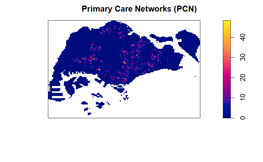
Bus Stops
busstop_bw <- density(busstop_ppp.km,
sigma = bw.diggle,
edge = TRUE,
kernel = "gaussian")
plot(busstop_bw, main = "Bus Stops")
Converting KDE Output into Grid Object
General Practitioner Clinics
gridded_gp_bw <- as.SpatialGridDataFrame.im(gp_bw)
spplot(gridded_gp_bw, main = "General Practitioners")
Hospitals
gridded_hospital_bw <- as.SpatialGridDataFrame.im(hospital_bw)
spplot(gridded_hospital_bw)
Polyclinics
gridded_poly_bw <- as.SpatialGridDataFrame.im(poly_bw)
spplot(gridded_poly_bw)
Nursing Homes
gridded_nursing_bw <- as.SpatialGridDataFrame.im(nursing_bw)
spplot(gridded_nursing_bw)
Bus Stops
gridded_busstop_bw <- as.SpatialGridDataFrame.im(busstop_bw)
spplot(gridded_busstop_bw)
CHAS
# gridded_chas_bw <- as.SpatialGridDataFrame.im(chas_bw)
# spplot(gridded_chas_bw)Converting Gridded Output into Raster
General Practitioner Clinics
kde_gp_bw_raster <- raster(gridded_gp_bw)
projection(kde_gp_bw_raster) <- CRS("+init=EPSG:3414")
kde_gp_bw_rasterclass : RasterLayer
dimensions : 128, 128, 16384 (nrow, ncol, ncell)
resolution : 0.419757, 0.2695907 (x, y)
extent : 2.667538, 56.39644, 15.74872, 50.25633 (xmin, xmax, ymin, ymax)
crs : +proj=tmerc +lat_0=1.36666666666667 +lon_0=103.833333333333 +k=1 +x_0=28001.642 +y_0=38744.572 +ellps=WGS84 +units=m +no_defs
source : memory
names : v
values : -1.971092e-14, 97.19965 (min, max)Hospitals
kde_hospital_bw_raster <- raster(gridded_hospital_bw)
projection(kde_hospital_bw_raster) <- CRS("+init=EPSG:3414")
kde_hospital_bw_rasterclass : RasterLayer
dimensions : 128, 128, 16384 (nrow, ncol, ncell)
resolution : 0.419757, 0.2695907 (x, y)
extent : 2.667538, 56.39644, 15.74872, 50.25633 (xmin, xmax, ymin, ymax)
crs : +proj=tmerc +lat_0=1.36666666666667 +lon_0=103.833333333333 +k=1 +x_0=28001.642 +y_0=38744.572 +ellps=WGS84 +units=m +no_defs
source : memory
names : v
values : -6.617214e-17, 0.6530283 (min, max)Polyclinics
kde_poly_bw_raster <- raster(gridded_poly_bw)
projection(kde_poly_bw_raster) <- CRS("+init=EPSG:3414")
kde_poly_bw_rasterclass : RasterLayer
dimensions : 128, 128, 16384 (nrow, ncol, ncell)
resolution : 0.419757, 0.2695907 (x, y)
extent : 2.667538, 56.39644, 15.74872, 50.25633 (xmin, xmax, ymin, ymax)
crs : +proj=tmerc +lat_0=1.36666666666667 +lon_0=103.833333333333 +k=1 +x_0=28001.642 +y_0=38744.572 +ellps=WGS84 +units=m +no_defs
source : memory
names : v
values : 1.253552e-17, 0.1114663 (min, max)Nursing Homes
kde_nursing_bw_raster <- raster(gridded_nursing_bw)
projection(kde_nursing_bw_raster) <- CRS("+init=EPSG:3414")
kde_nursing_bw_rasterclass : RasterLayer
dimensions : 128, 128, 16384 (nrow, ncol, ncell)
resolution : 0.419757, 0.2695907 (x, y)
extent : 2.667538, 56.39644, 15.74872, 50.25633 (xmin, xmax, ymin, ymax)
crs : +proj=tmerc +lat_0=1.36666666666667 +lon_0=103.833333333333 +k=1 +x_0=28001.642 +y_0=38744.572 +ellps=WGS84 +units=m +no_defs
source : memory
names : v
values : -1.246191e-16, 0.87121 (min, max)Bus Stops
kde_busstop_bw_raster <- raster(gridded_busstop_bw)
projection(kde_busstop_bw_raster) <- CRS("+init=EPSG:3414")
kde_busstop_bw_rasterclass : RasterLayer
dimensions : 128, 128, 16384 (nrow, ncol, ncell)
resolution : 0.419757, 0.2695907 (x, y)
extent : 2.667538, 56.39644, 15.74872, 50.25633 (xmin, xmax, ymin, ymax)
crs : +proj=tmerc +lat_0=1.36666666666667 +lon_0=103.833333333333 +k=1 +x_0=28001.642 +y_0=38744.572 +ellps=WGS84 +units=m +no_defs
source : memory
names : v
values : -1.15015e-14, 46.68152 (min, max)CHAS
kde_busstop_bw_raster <- raster(gridded_busstop_bw)
projection(kde_busstop_bw_raster) <- CRS("+init=EPSG:3414")
kde_busstop_bw_rasterclass : RasterLayer
dimensions : 128, 128, 16384 (nrow, ncol, ncell)
resolution : 0.419757, 0.2695907 (x, y)
extent : 2.667538, 56.39644, 15.74872, 50.25633 (xmin, xmax, ymin, ymax)
crs : +proj=tmerc +lat_0=1.36666666666667 +lon_0=103.833333333333 +k=1 +x_0=28001.642 +y_0=38744.572 +ellps=WGS84 +units=m +no_defs
source : memory
names : v
values : -1.15015e-14, 46.68152 (min, max)Visualisation
General Practitioner Clinics
tm_shape(kde_gp_bw_raster) +
tm_raster("v") +
tm_layout(legend.position = c("right", "bottom"), frame = FALSE)Variable(s) "v" contains positive and negative values, so midpoint is set to 0. Set midpoint = NA to show the full spectrum of the color palette.
Hospitals
tm_shape(kde_hospital_bw_raster) +
tm_raster("v") +
tm_layout(legend.position = c("right", "bottom"), frame = FALSE)Variable(s) "v" contains positive and negative values, so midpoint is set to 0. Set midpoint = NA to show the full spectrum of the color palette.
Polyclinics
tm_shape(kde_poly_bw_raster) +
tm_raster("v") +
tm_layout(legend.position = c("right", "bottom"), frame = FALSE)
Nursing Homes
tm_shape(kde_nursing_bw_raster) +
tm_raster("v") +
tm_layout(legend.position = c("right", "bottom"), frame = FALSE)Variable(s) "v" contains positive and negative values, so midpoint is set to 0. Set midpoint = NA to show the full spectrum of the color palette.
Bus Stops
tm_shape(kde_busstop_bw_raster) +
tm_raster("v") +
tm_layout(legend.position = c("right", "bottom"), frame = FALSE)Variable(s) "v" contains positive and negative values, so midpoint is set to 0. Set midpoint = NA to show the full spectrum of the color palette.
CHAS Clinics
chas_bw <- density(chas_ppp.km,
sigma = bw.diggle,
edge = TRUE,
kernel = "gaussian")
plot(chas_bw, main = "CHAS Clinics")
tm_shape(kde_busstop_bw_raster) +
tm_raster("v") +
tm_layout(legend.position = c("right", "bottom"), frame = FALSE)Variable(s) "v" contains positive and negative values, so midpoint is set to 0. Set midpoint = NA to show the full spectrum of the color palette.
Nearest Neighbour Analysis
General Practitioner Clinics
Ho = The distribution of general practitioner clinics are randomly distributed.
H1 = The distribution of general practitioner clinics are not randomly distributed.
With the p-value lower than the alpha value of 0.05, we reject the null hypothesis and accept that general practitioner clinics are not randomly distributed.
clarkevans.test(gp_ppp.km,
correction = "none",
clipregion = "mpsz_owin",
alternative = c("clustered"),
nsim = 99)
Clark-Evans test
No edge correction
Monte Carlo test based on 99 simulations of CSR with fixed n
data: gp_ppp.km
R = 0.34517, p-value = 0.01
alternative hypothesis: clustered (R < 1)Hospitals
Ho = The distribution of hospitals are randomly distributed.
H1 = The distribution of hospitals are not randomly distributed.
With the p-value lower than the alpha value of 0.05, we reject the null hypothesis and accept that hospitals are not randomly distributed.
clarkevans.test(hospital_ppp.km,
correction = "none",
clipregion = "mpsz_owin",
alternative = c("clustered"),
nsim = 99)
Clark-Evans test
No edge correction
Monte Carlo test based on 99 simulations of CSR with fixed n
data: hospital_ppp.km
R = 0.45977, p-value = 0.01
alternative hypothesis: clustered (R < 1)Polyclinics
Ho = The distribution of polyclinics are randomly distributed.
H1 = The distribution of polyclinics are not randomly distributed.
With the p-value above than the alpha value of 0.05, we accept the null hypothesis and accept that polyclinics are randomly distributed.
clarkevans.test(poly_ppp.km,
correction = "none",
clipregion = "mpsz_owin",
alternative = c("clustered"),
nsim = 99)
Clark-Evans test
No edge correction
Monte Carlo test based on 99 simulations of CSR with fixed n
data: poly_ppp.km
R = 1.0189, p-value = 0.14
alternative hypothesis: clustered (R < 1)Nursing Homes
Ho = The distribution of nursing homes are randomly distributed.
H1 = The distribution of nursing homes are not randomly distributed.
With the p-value lower than the alpha value of 0.05, we reject the null hypothesis and accept that nursing homes are not randomly distributed.
clarkevans.test(nursing_ppp.km,
correction = "none",
clipregion = "mpsz_owin",
alternative = c("clustered"),
nsim = 99)
Clark-Evans test
No edge correction
Monte Carlo test based on 99 simulations of CSR with fixed n
data: nursing_ppp.km
R = 0.71101, p-value = 0.01
alternative hypothesis: clustered (R < 1)CHAS Clinics
Ho = The distribution of CHAS clinics are randomly distributed.
H1 = The distribution of CHAS clinics are not randomly distributed.
With the p-value lower than the alpha value of 0.05, we reject the null hypothesis and accept that CHAS clinics are not randomly distributed.
clarkevans.test(chas_ppp.km,
correction = "none",
clipregion = "mpsz_owin",
alternative = c("clustered"),
nsim = 99)
Clark-Evans test
No edge correction
Monte Carlo test based on 99 simulations of CSR with fixed n
data: chas_ppp.km
R = 0.48715, p-value = 0.01
alternative hypothesis: clustered (R < 1)Modelling Geographical Accessibility
PCN_Clinics <- st_read(dsn = "data/geospatial/PCN Network Clinics Shapefile",
layer = "PCN Network Clinics") %>%
st_transform(crs = 3414)Reading layer `PCN Network Clinics' from data source
`C:\deadline2359\IS415-Project\posts\data_cleaning\data\geospatial\PCN Network Clinics Shapefile'
using driver `ESRI Shapefile'
replacing null geometries with empty geometries
Simple feature collection with 828 features and 20 fields (with 1 geometry empty)
Geometry type: POINT
Dimension: XY
Bounding box: xmin: 4985.536 ymin: 26424.19 xmax: 45002.49 ymax: 48986.95
Projected CRS: SVY21 / Singapore TM